Monitoring Throughput Trends with the One Degree Imager and PPA
All images taken with the WIYN One Degree Imager are stored and calibrated within the ODI Pipeline, Portal, and Archive (PPA) system. Within PPA, the data are calibrated with a ODI quick reduce data pipeline; calibrated images and their metadata (basic information about where the telescope was pointed, but also photometric depth and other derived information) can then be searched and downloaded from the PPA system.
This pool of metadata is a great tool to understand the long-term behaviour of the One Degree Imager. In the example here I analyze trends in the throughput of the telescope and instrument system over three years. Let’s get started:
Extracting metadata from the ODI Archive
To access actual imaging data, an account for the PPA system is required. But for a query for meta data, no such thing is required. In the login screen, we select “Browse Archive”, and search for all “Operator Calibrated Images”. In order to select other specific columns that I want for this study, I still need to log in. Here is how the screen looks like:
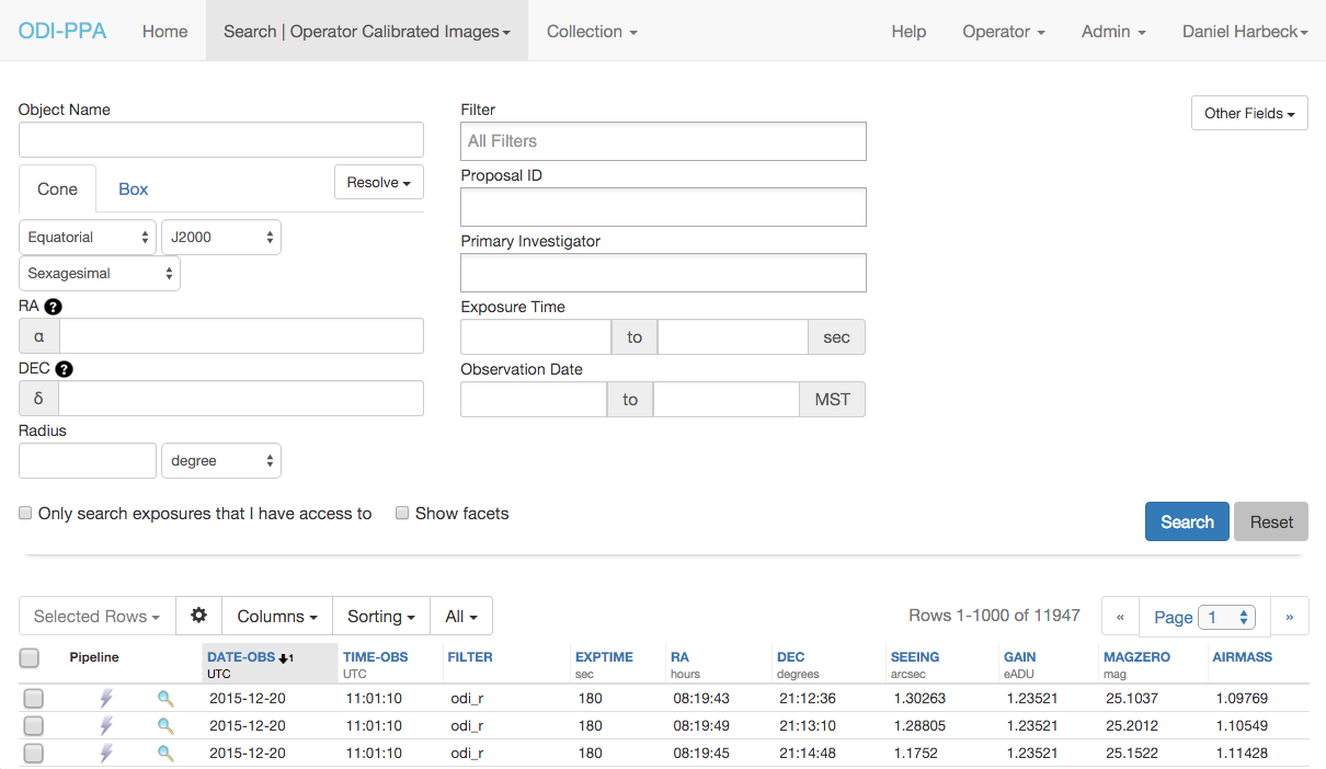
OK, this is a long list of nearly 12000 images. I wanted the trends for all data ever taken with ODI, so I did not restrict the search. The little “All…” button above the search results will reveal an export function, which allows us to download all the selected metadata for all the 12000 images. Once we have that on our drive, and after a short vi session to rectify a few things here and there, we are ready for a data analysis session to look at any trends in the data.
Exploring the data with pyhton
My weapon of choice to look at data is python, in a jupyter session. Let’s read in the data. There is a bit overhead involved to read in dates and times and strings as such:
%matplotlib inline
import matplotlib.pyplot as plt
import matplotlib
import numpy as np
from datetime import datetime, date, time, timedelta
mydata = np.loadtxt ("allodi_022016.dat" , delimiter=', ',
          dtype={ 'names': ('date', 'time', 'filter', 'exptime', 'ra', 'dec', 'seeing', 'gain', 'magzero', 'airmass'),
          'formats': (object, object, object, np.float, np.float, np.float, np.float, np.float, np.float, np.float)},
          converters={0: lambda x: datetime.strptime(x,"%Y-%m-%d"),
          1: lambda x: datetime.strptime(x,"%H:%M:%S"),
          2: lambda x: np.str(x)},
          unpack = True)
# adjust the date field to contain both date and time in one datetime object
mydata[0] = mydata[0] + (mydata[1] - datetime(1900,1,1))

# Gain correct data; multiple epochs might have seen
#      different flat field normalisataions
mydata[8] = mydata[8] + np.log10( mydata[7] )
Next, let’s define a plotting function for a given filter. This plotting function will take an airmass correction term as a parameter so we end up with a photometric zeropoint corrected for zero airmasses.
# Plot the long-term trend in a given filter.
def plotForFilter (filter, xterm, refmag=28):
    cond = mydata[2] == filter
    fdate = mydata[0][cond]
    fmag = mydata[8][cond]
    fx = mydata[9][cond]

    fmag = fmag + xterm * fx - refmag
    fig, ax = plt.subplots(1)
    fig.autofmt_xdate()
    ax.grid (True)
    plt.plot (fdate, fmag, ".")
    plt.ylim (-2,0.5)
    plt.ylabel ("dZP [e-/s], X=0")
    plt.title ("Zeropint deviation for %s" % (filter))
    plt.savefig ("odizp_%s.pdf" % (filter))
    plt.show()
And lastly, do some plots:
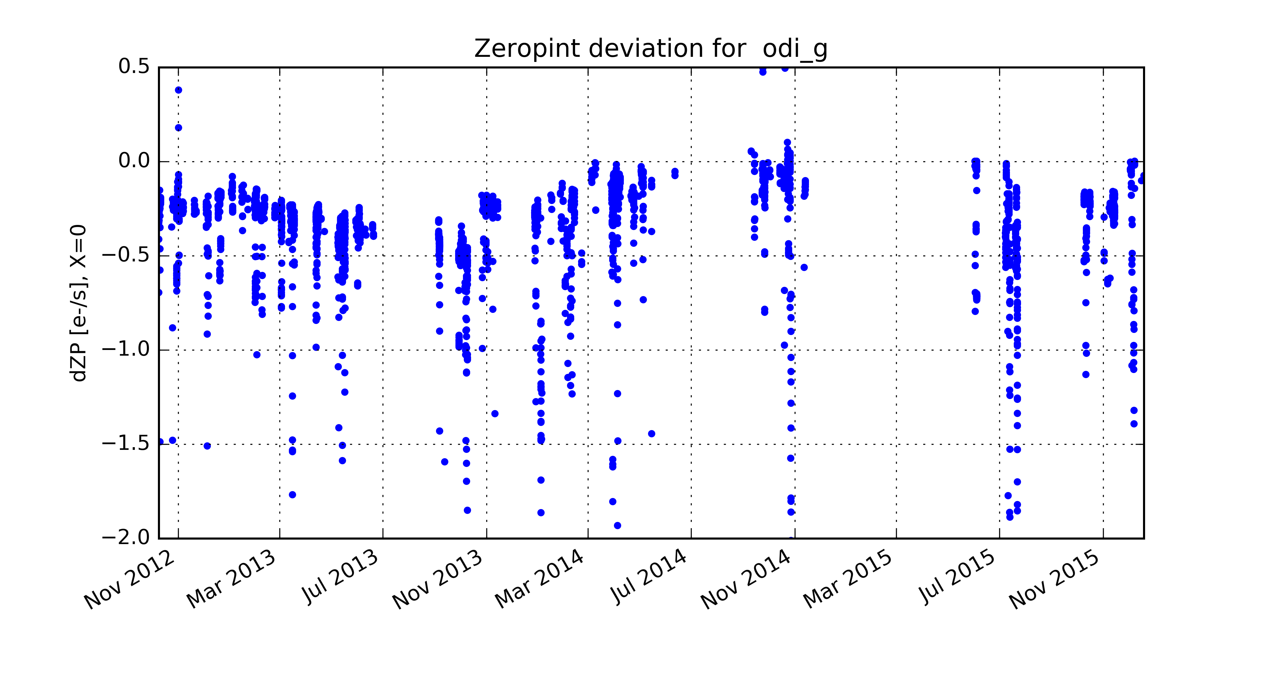
plotForFilter ('odi_g', 0.2, 26.7)
The output is a figure showing the relative photometric zeropoint, i.e., the throughput of the telescope and instrument, over a time span of three years:
Interpretation of long-term trends
There are a few very interesting conclusions one can take from the above figure:
-
There was a systematic degradation in throughput during the first year of operations, with a clear improvement occurring during the first few month of 2014.
Why? Shocked by the diminishing throughput of ODI, we implemented a bi-weekly telescope mirror C02 snow cleaning and washing program. -
There is a slight improvement in the throughput in the second half of 2014. During the summer break, we recoated the telescope mirrors, which improved their reflectivity / reduced light scattering.
-
Around November 2015, there was a significant drop in the measured throughput - this was attributed to condensation residue on the dewar window, which was mitigated for the December 2015 data - one can clearly see the recovery of throughput there.
-
In December 2015, the system throughput is comparable to the system throughput after realuminizing the telescope’s primary mirror. The ongoing mirror cleaning proves to be working and recoating of the mirrors might not be required in 2016.
Conclusion
Having all ODI data stored and processed in a single place has opened the door to understand long-term trends of the instrument and telescope system. The example of monitoring the throughput of ODI allows the operating team to make informed, evidence-based decision on mirror cleaning and coating schedules.